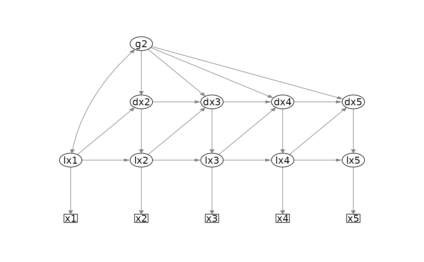
Plot simplified path diagram of univariate and bivariate latent change score models

Note that the following three arguments are needed to create a plot (see below for more details):

lavaan_object: the lavaan fit object needs to be specified together with a
lcsm: a string indicating whether the latent change score model is "univariate" or "bivariate", and
lavaan_syntax: a separate object with the lavaan syntax as a string

Usage

plot_lcsm(
  lavaan_object,
  layout = NULL,
  lavaan_syntax = NULL,
  return_layout_from_lavaan_syntax = FALSE,
  lcsm = c("univariate", "bivariate"),
  lcsm_colours = FALSE,
  curve_covar = 0.5,
  what = "path",
  whatLabels = "est",
  edge.width = 1,
  node.width = 1,
  border.width = 1,
  fixedStyle = 1,
  freeStyle = 1,
  residuals = FALSE,
  label.scale = FALSE,
  sizeMan = 3,
  sizeLat = 5,
  intercepts = FALSE,
  fade = FALSE,
  nCharNodes = 0,
  nCharEdges = 0,
  edge.label.cex = 0.5,
  ...
)

Arguments

lavaan_object: lavaan object of a univariate or bivariate latent change score model.
layout: Matrix, specifying number and location of manifest and latent variables of LCS model specified in lavaan_object.
lavaan_syntax: String, lavaan syntax of the lavaan object specified in lavaan_object. If lavaan_syntax is provided a layout matrix will be generated automatically.
return_layout_from_lavaan_syntax: Logical, if TRUE and lavaan_syntax is provided, the layout matrix generated for semPaths will be returned for inspection of further customisation.
lcsm: String, specifying whether lavaan_object represent a "univariate" or "bivariate" LCS model.
lcsm_colours: Logical, if TRUE the following colours will be used to highlight different parts of the model: Observed variables (White); Latent true scores (Green); Latent change scores (Blue) ; Change factors (Yellow).
curve_covar: See semPaths.
what: See semPlot. "path" to show unweighted grey edges, "par" to show parameter estimates as weighted (green/red) edges
whatLabels: See semPaths. "label" to show edge names as label, "est" for parameter estimates, "hide" to hide edge labels.
edge.width: See semPaths.
node.width: See semPaths.
border.width: See semPaths.
fixedStyle: See semPaths.
freeStyle: See semPaths.
residuals: See semPaths.
label.scale: See semPaths.
sizeMan: See semPaths.
sizeLat: See semPaths.
intercepts: See semPaths.
fade: See semPaths.
nCharNodes: See semPaths.
nCharEdges: See semPaths.
edge.label.cex: See semPaths.
...: Other arguments passed on to semPaths.

Value

Plot

References

Sacha Epskamp (2019). semPlot: Path Diagrams and Visual Analysis of Various SEM Packages' Output. R package version 1.1.1. https://CRAN.R-project.org/package=semPlot/

Examples

# Simplified plot of univariate lcsm
lavaan_syntax_uni <- fit_uni_lcsm(
  data = data_bi_lcsm,
  var = c("x1", "x2", "x3", "x4", "x5"),
  model = list(
    alpha_constant = TRUE,
    beta = TRUE,
    phi = TRUE
  ),
  return_lavaan_syntax = TRUE,
  return_lavaan_syntax_string = TRUE
)

lavaan_object_uni <- fit_uni_lcsm(
  data = data_bi_lcsm,
  var = c("x1", "x2", "x3", "x4", "x5"),
  model = list(
    alpha_constant = TRUE,
    beta = TRUE,
    phi = TRUE
  )
)

plot_lcsm(
  lavaan_object = lavaan_object_uni,
  what = "cons", whatLabels = "invisible",
  lavaan_syntax = lavaan_syntax_uni,
  lcsm = "univariate"
)

if (FALSE) {
# Simplified plot of bivariate lcsm
lavaan_syntax_bi <- fit_bi_lcsm(
  data = data_bi_lcsm,
  var_x = c("x1", "x2", "x3", "x4", "x5"),
  var_y = c("y1", "y2", "y3", "y4", "y5"),
  model_x = list(
    alpha_constant = TRUE,
    beta = TRUE,
    phi = TRUE
  ),
  model_y = list(
    alpha_constant = TRUE,
    beta = TRUE,
    phi = TRUE
  ),
  coupling = list(
    delta_lag_xy = TRUE,
    delta_lag_yx = TRUE
  ),
  return_lavaan_syntax = TRUE,
  return_lavaan_syntax_string = TRUE
)

lavaan_object_bi <- fit_bi_lcsm(
  data = data_bi_lcsm,
  var_x = c("x1", "x2", "x3", "x4", "x5"),
  var_y = c("y1", "y2", "y3", "y4", "y5"),
  model_x = list(
    alpha_constant = TRUE,
    beta = TRUE,
    phi = TRUE
  ),
  model_y = list(
    alpha_constant = TRUE,
    beta = TRUE,
    phi = TRUE
  ),
  coupling = list(
    delta_lag_xy = TRUE,
    delta_lag_yx = TRUE
  )
)

plot_lcsm(
  lavaan_object = lavaan_object_bi,
  what = "cons", whatLabels = "invisible",
  lavaan_syntax = lavaan_syntax_bi,
  lcsm = "bivariate"
)
}